pdpipe ❤️ sklearn
pdpipe has strong existing tools to enable integration with scikit-learn models. Besides [stages integrating important scikit-learn transformations], it boasts a custom class that allows the integration of pdpipe pipelines and sklearn estimator into a single parameterized pipeline-and-model object, the parameters of which can be optimized jointly.
.. [stages integrating important scikit-learn transformations] https://pdpipe.readthedocs.io/en/latest/reference/sklearn/
The PdPipelineAndSklearnEstimator class
To create such custom joint object, you can extend the PdPipelineAndSklearnEstimator. Here's an example:
from typing import Optional
import pdpipe as pdp
from pdpipe.skintegrate import PdPipelineAndSklearnEstimator
from sklearn.linear_model import LogisticRegression

class MyPipelineAndModel(PdPipelineAndSklearnEstimator):

    def __init__(
        self,
        savings_max_val: Optional[int] = 100,
        drop_gender: Optional[bool] = False,
        scale_numeric: Optional[bool] = False,
        ohencode_country: Optional[bool] = True,
        savings_bin_val: Optional[int] = None,
        fit_intercept: Optional[bool] = True,
    ):
        self.savings_max_val = savings_max_val
        self.drop_gender = drop_gender
        self.scale_numeric = scale_numeric
        self.ohencode_country = ohencode_country
        self.savings_bin_val = savings_bin_val
        self.fit_intercept = fit_intercept
        cols_to_drop = []
        stages = [
            pdp.ColDrop(['Name', 'Quote'], errors='ignore'),
            pdp.RowDrop({'Savings': lambda x: x > savings_max_val}),
        ]
        if savings_bin_val:
            stages.append(pdp.Bin({'Savings': [savings_bin_val]}, drop=False))
            stages.append(pdp.Encode('Savings_bin'))
        if scale_numeric:
            stages.append(pdp.Scale('MinMaxScaler'))
        if drop_gender:
            cols_to_drop.append('Gender')
        else:
            stages.append(pdp.Encode('Gender'))
        if ohencode_country:
            stages.append(pdp.OneHotEncode('Country'))
        else:
            cols_to_drop.append('Country')
        stages.append(pdp.ColDrop(cols_to_drop, errors='ignore'))
        pline = pdp.PdPipeline(stages)
        model = LogisticRegression(fit_intercept=fit_intercept)
        super().__init__(pipeline=pline, estimator=model)
Objects of this type are now initialized by detailing both pipeline parameters and model parameters:
mp = MyPipelineAndModel(
    savings_max_val=101,
    drop_gender=True,
    scale_numeric=True,
    ohencode_country=True,
    savings_bin_val=1,
    fit_intercept=True,
)
The initialized object is now a pipeline followed by a LogisticRegression model.
The inner pipeline object can be accessed using the mp.pipeline attribute, while the model can be accessed using the mp.estimator attribute.
Using pipeline-estimator joint objects
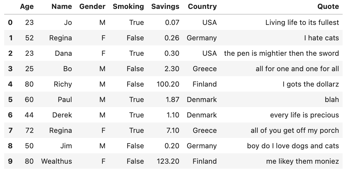
Let's look at an example dataframe:
import pandas as pd

df = pd.DataFrame(
    data=[
        [23, 'Jo', 'M', True, 0.07, 'USA', 'Living life to its fullest'],
        [52, 'Regina', 'F', False, 0.26, 'Germany', 'I hate cats'],
        [23, 'Dana', 'F', True, 0.3, 'USA', 'the pen is mightier then the sword'],
        [25, 'Bo', 'M', False, 2.3, 'Greece', 'all for one and one for all'],
        [80, 'Richy', 'M', False, 100.2, 'Finland', 'I gots the dollarz'],
        [60, 'Paul', 'M', True, 1.87, 'Denmark', 'blah'],
        [44, 'Derek', 'M', True, 1.1, 'Denmark', 'every life is precious'],
        [72, 'Regina', 'F', True, 7.1, 'Greece', 'all of you get off my porch'],
        [50, 'Jim', 'M', False, 0.2, 'Germany', 'boy do I love dogs and cats'],
        [80, 'Wealthus', 'F', False, 123.2, 'Finland', 'me likey them moniez'],
    ],
    columns=['Age', 'Name', 'Gender', 'Smoking', 'Savings', 'Country', 'Quote'],
)
This is how it looks:
Let's divide it to the X and y of our supervised learning problem - learning to predict smokers:
X_lbls = ['Age', 'Gender', 'Savings', 'Country']
all_X = df[X_lbls]
all_y = df['Smoking']
train_df = df.iloc[0:6]
train_X = train_df[X_lbls]
train_y = train_df['Smoking']
test_df = df.iloc[6:]
test_X = test_df[X_lbls]
test_y = test_df['Smoking']
Now, to get an idea what will happen inside the joint object when we fit on train_X, train_y and predict on test_X, test_y, let's play with the internals. Insie, on fit time, the pipeline will be called with pipeline.fit_transform(train_X, train_y. Let's call it:
This yields, for the transformed X:

The pipeline can now be used to transform test_X, test_y:

When using the object itself, will call its sklearn-compliant methods: First, calling mp.fit(train_X, train_y) and then mp.predict(test_X). Recall, this class extends sklearn.BaseEstimator abstract base class, and thus plays nice with scikit-learn code.
Grid search cross validation with pipeline-object models
We can also joinly optimize the parameters of both the pipeline and model using sklearn's GridSearchCV:
from sklearn.model_selection import GridSearchCV

gcv = GridSearchCV(
    estimator=mp,
    param_grid={
        'savings_max_val': [99, 101],
        'scale_numeric': [True, False],
        'drop_gender': [True, False],
        'ohencode_country': [True, False],
    },
    cv=3,
)
Our joint pipeline-model is successfully embedded into the GridSearchCV object:
>>> gcv
GridSearchCV(cv=3,
             ('estimator', <PdPipeline -> LogisticRegression>),
             param_grid={'drop_gender': [True, False],
                         'ohencode_country': [True, False],
                         'savings_max_val': [99, 101],
                         'scale_numeric': [True, False]})
We can now fit our GridSearchCV object and look at what was found (we truncate most of the long output):
>>> gcv.fit(all_x, all_y)
>>> gcv.cv_results_
{'mean_fit_time': array([0.01805862, 0.02602871, 0.01143765, 0.01497038, 0.01344951,
        0.01279736, 0.01329573, 0.01088969, 0.01029619, 0.01027075,
        0.01030358, 0.01006969, 0.01032559, 0.00969656, 0.01018016,
        0.01164174]),
 'std_fit_time': array([2.18801548e-03, 1.98170580e-02, 2.25330743e-04, 1.24616889e-03,
        4.48451862e-04, 2.54838793e-04, 1.36396307e-03, 9.32612305e-04,
        1.79914724e-04, 1.08602622e-04, 9.75366752e-05, 5.21974790e-04,
        3.32276720e-04, 2.21513857e-04, 4.10991280e-04, 1.38408821e-03]),
 'mean_score_time': array([0.01330503, 0.01307933, 0.00831469, 0.01016466, 0.01000388,
        0.01001596, 0.01021091, 0.00968703, 0.00961073, 0.00952029,
        0.00930103, 0.00886997, 0.00903908, 0.00896827, 0.00967216,
        0.00930333]),
 'std_score_time': array([1.13176156e-03, 6.24168155e-03, 2.63902576e-04, 6.38240356e-04,
        4.58783486e-04, 6.55998340e-04, 1.96695312e-04, 1.49338914e-04,
        5.19397646e-04, 5.46878381e-05, 1.20865496e-04, 1.90029961e-04,
        7.80427529e-05, 1.09872486e-04, 5.77189107e-04, 6.72587756e-04]),
 'param_drop_gender': masked_array(data=[True, True, True, True, True, True, True, True, False,
                    False, False, False, False, False, False, False],
              mask=[False, False, False, False, False, False, False, False,
                    False, False, False, False, False, False, False, False],
        fill_value='?',
             dtype=object),
 'param_ohencode_country': masked_array(data=[True, True, True, True, False, False, False, False,
                    True, True, True, True, False, False, False, False],
              mask=[False, False, False, False, False, False, False, False,
                    False, False, False, False, False, False, False, False],
        fill_value='?',
             dtype=object),
 'param_savings_max_val': masked_array(data=[99, 99, 101, 101, 99, 99, 101, 101, 99, 99, 101, 101,
                    99, 99, 101, 101],
              mask=[False, False, False, False, False, False, False, False,
                    False, False, False, False, False, False, False, False],
        fill_value='?',
             dtype=object),
 'param_scale_numeric': masked_array(data=[True, False, True, False, True, False, True, False,
                    True, False, True, False, True, False, True, False],
              mask=[False, False, False, False, False, False, False, False,
                    False, False, False, False, False, False, False, False],
        fill_value='?',
             dtype=object),
 'params': [{'drop_gender': True,
   'ohencode_country': True,
   'savings_max_val': 99,
   'scale_numeric': True},
   ...
  {'drop_gender': False,
   'ohencode_country': False,
   'savings_max_val': 101,
   'scale_numeric': False}],
 'split0_test_score': array([0.75, 0.75, 0.75, 0.75, 0.75, 0.75, 0.75, 0.75, 0.75, 0.75, 0.75,
        0.75, 0.75, 0.75, 0.75, 0.75]),
 'split1_test_score': array([0., 0., 0., 0., 0., 0., 0., 0., 0., 0., 0., 0., 0., 0., 0., 0.]),
 'split2_test_score': array([0.5, 0.5, 0.5, 0.5, 0.5, 0.5, 0.5, 0.5, 0.5, 0.5, 0.5, 0.5, 0.5,
        0.5, 0.5, 0.5]),
 'mean_test_score': array([0.41666667, 0.41666667, 0.41666667, 0.41666667, 0.41666667,
        0.41666667, 0.41666667, 0.41666667, 0.41666667, 0.41666667,
        0.41666667, 0.41666667, 0.41666667, 0.41666667, 0.41666667,
        0.41666667]),
 'std_test_score': array([0.31180478, 0.31180478, 0.31180478, 0.31180478, 0.31180478,
        0.31180478, 0.31180478, 0.31180478, 0.31180478, 0.31180478,
        0.31180478, 0.31180478, 0.31180478, 0.31180478, 0.31180478,
        0.31180478]),
 'rank_test_score': array([1, 1, 1, 1, 1, 1, 1, 1, 1, 1, 1, 1, 1, 1, 1, 1], dtype=int32)}
The best estimator is itself, of course, a pipeline-estimator object, and we got the best parameters for both the pipeline and the model:
>>> gcv.best_estimator_
<PdPipeline -> LogisticRegression>
>>> gcv.best_score_
0.4166666666666667
>>> gcv.best_params_
{'drop_gender': True,
 'ohencode_country': True,
 'savings_max_val': 99,
 'scale_numeric': True}
Working with custom scorers
The PdPipelineAndSklearnEstimator class implements the score method in a way that makes everything jive with sklearn. To work with custom scores when performing grid search cross validation with sklearn, you must wrap sklearn scorers and scoring functions into PdPipeScorer objects for them to work with the joint pipeline-estimator objects:
>>> from sklearn.metrics import fbeta_score, make_scorer
>>> from pdpipe.skintegrate import pdpipe_scorer_from_sklearn_scorer
>>> ftwo_scorer = make_scorer(fbeta_score, beta=2)
>>> my_scorer = pdpipe_scorer_from_sklearn_scorer(ftwo_scorer)
>>> my_scorer
<PdPipeScorer: make_scorer(fbeta_score, beta=2)>
You can now use this wrapped scorer with GridSearchCV:
gcv = GridSearchCV(
    estimator=mp,
    param_grid={
        'savings_max_val': [99, 101],
        'scale_numeric': [True, False],
        'drop_gender': [True, False],
        'ohencode_country': [True, False],
    },
    cv=3,
    scoring=my_scorer,
)
That's it!
Getting help
Remember you can get help on our Gitter chat or on our GitHub Discussions forum.